Representational Difference Distillation
Divin Irakiza, AbdulKarim Mugisha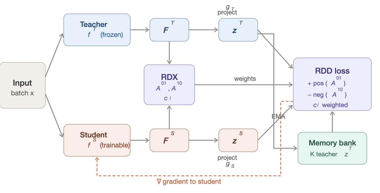
Figure 1: A shared input batch passes through the frozen teacher and the trainable student , producing features and . The RDX diagnostic computes two asymmetric affinity matrices from rank-normalized distances: captures teacher-unique structure and captures student-unique structure, along with a per-sample confusion score . Both feature sets are projected onto a shared hypersphere via and . The RDD loss selects positives using , weights negatives by , draws additional negatives from a momentum-updated memory bank, and scales each anchor's loss by . Gradients flow only to the student.
#1. Background & Related Work
KD transfers the learned representations of a large teacher model into a smaller student model. Since the original KL-divergence formulation, 1 which trains the student to match the teacher's softened output distribution. However, a wave of methods has moved beyond matching pointwise logits to care about structural representations instead. Relational methods like RKD 2 penalize differences in pairwise distance between samples. Contrastive methods like CRD 3 and RRD 4 maximize mutual information between teacher and student representations using negative samples. These methods consistently outperform pointwise approaches which hinted to us that the geometric structure in the latent space is a strong signal for distillation than raw activation matching. It is noteworthy that these methods treat every pair is treated equally. The contrastive loss spends the same gradient on sample pairs the student has already captured and pairs where the student is completely lost. We hypothesized that representational interpretability methods could diagnose where the student is wrong and direct the distillation signal there, yielding better performance from the same training budget.#1.2 Representational Difference Explanations
Kondapaneni et al introduced RDX to effectively explain contrasting model representations. 5 Given two embedding matrices over the same data, RDX computes rank-normalized pairwise distances and applies a locally-biased difference function that amplifies disagreements between nearby samples while suppressing those between distant ones. The result is an affinity matrix that reveals groups of samples one model considers similar but the other does not. Our repurposed its core machinery (rank normalization + locally-biased difference) as a supervision signal inside a distillation loss. Instead of producing post-hoc explanations, we use RDX to compute per-sample confusion weights that modulate the distillation gradient in real time. To our knowledge, this is the first application of representational difference analysis as a direct component of a distillation objective.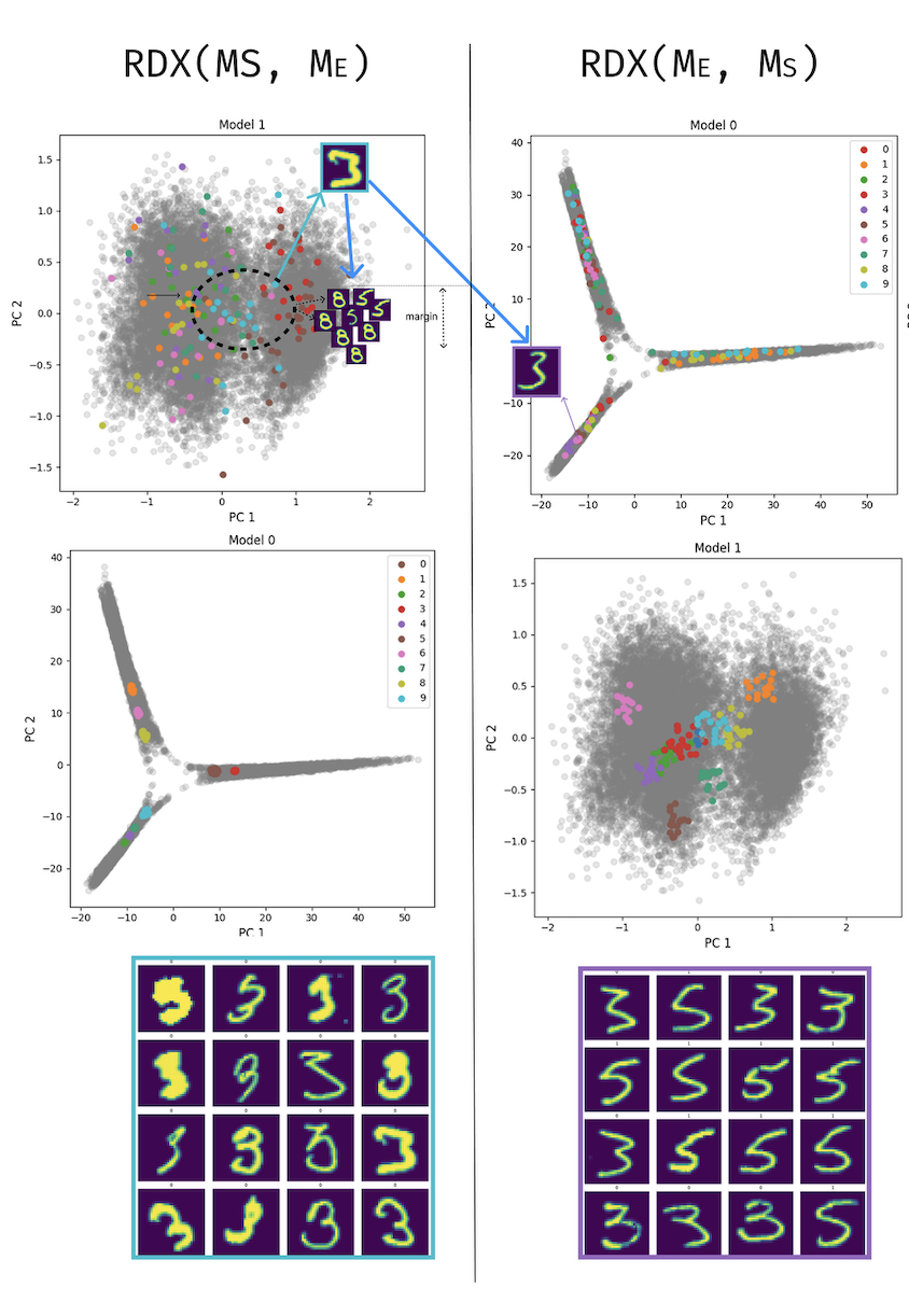
Figure 2: RDX-guided selection on MNIST digits 3, 5, 8 with a student model and expert model . Left: reveals clusters unique to the student: samples the student groups tightly (cyan cluster, top-left PCA) that the expert separates (top-right PCA). These are the hard negatives: the student wrongly merges 3s, 5s, and 8s that the teacher distinguishes, identified by high in the affinity matrix. Right: reveals structure unique to the teacher: samples the expert clusters coher- ently that the student scatters. These inform positive selection: teacher-close pairs the student has yet to learn. Bottom grids show the corresponding image samples for each direction.
#2. Approach
We propose Representational Difference Distillation (RDD), a knowledge distillation framework that uses representational difference analysis to focus the distillation loss where the teacher and student structurally disagree.#2.1 Identify Representational Misalignment
For every pair of samples , compute ranks in teacher-space and student-space, then measure how much they disagree:Negative values mean the student over-groups and ; positive values mean the student has an alignment gap to close. This becomes two asymmetric affinity matrices: (teacher-unique structure), (student-unique structure), and a per-sample confusion score .
#2.2 Guided Contrastive Loss
We build on CRD's memory-bank contrastive setup but make two changes 3. Positives are selected via , the strongest teacher-unique neighbor for each anchor. Negatives are drawn from a top- pool ranked by , samples the student wrongly merges. Each anchor's contrastive loss is then scaled by its normalized confusion score:
#2.3 Training Objective
The final training loss is:
Standard cross-entropy, standard KD, plus our RDX-weighted contrastive term.
#3. Results
We evaluate on CIFAR-100 (50k train / 10k test, 100 classes) using the resnet32x4 → resnet8x4 teacher–student pair, following the protocol from CRD. All methods KD, RKD, CRD, and ours have: SGD with momentum 0.9, weight decay , initial learning rate 0.05 decayed by at epochs 150, 180, and 210, for 240 total epochs at batch size 64. For the RDX diagnostic we set , ; the combined loss weights are , , . All results are averaged over 5 runs.#3.1 Naive Sampling
Our first instinct was to use RDX as a signal for online batch selection that is: only train on the samples where teacher and student disagree most. There is good precedent for active sampling methods like RHO Loss, 6 and we were initially optimistic. We beat random sampling by a small margin as shown in Figure 3. But we could not beat any distillation baseline. RDD sampling had 59.49%, substantially below KD (72.93%), CRD (75.45%), and everything else. The reason, in hindsight, is obvious, by restricting training to the easiest RDX-ranked samples, the student only ever sees the portion of the data where teacher and student already agree. It never encounters the challenging boundary cases that drive representation refinement. The student converges quickly to a solution that handles easy samples well but generalizes poorly.
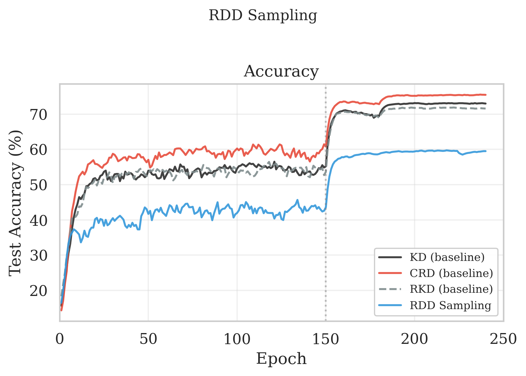
Figure 3: CIFAR-100 resnet32x4→resnet8x4 test accuracy. RDD sampling trains on an RDX-ranked subset (easy→hard); the subset is recomputed every Repochs. Curves shown for KD, CRD, RKD, and RDD sampling.
#3.2 Curriculum Learning
Instead of restricting to easy RDX-ranked samples, we start with them and gradually introduce harder ones through curriculum learning. 7 RDX confusion scores give us a principled difficulty ranking derived from actual structural disagreement. RDD curriculum reached 72.96%, matching KD, but falling short of CRD. The reason for this was that during the initial phase when only the easiest 30% of samples are available, the student learns a reasonable but incomplete representation. As harder samples come in, the student must reorganize its feature space to accommodate them, causing a visible slowdown around epochs 60-100. By epoch 150 all samples are active and performance catches up to KD.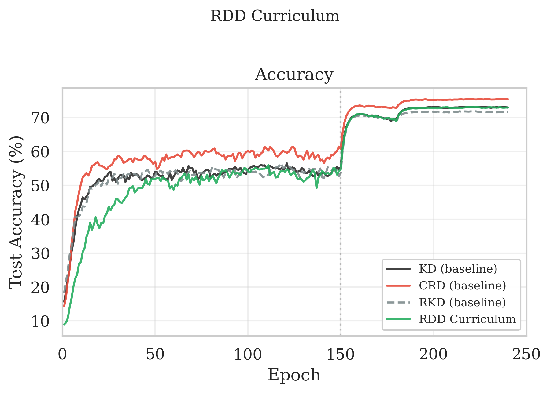
Figure 4: CIFAR-100 resnet32x4→resnet8x4 test accuracy. RDD curriculum uses RDX difficulty scores to start from a fraction of the easiest samples and linearly ramps to full data over epochs. Curves shown for KD, CRD, RKD, and RDD curriculum
#3.3 RDX-Weighted Supervision
Our final method, RDX-weighted supervision achieves the strongest representation alignment. Our method achieves 75.58% test accuracy, outperforming CRD (75.45%), KD (72.93%), and RKD (71.55%) as shown in Figure 5. We attribute this gain to the asymmetric use of the two RDX affinity matrices. While CRD treats all negatives uniformly, RDD concentrates gradient on the specific memory bank negatives that identifies as wrongly merged by the student. RDD allocates the majority of its gradient budget to the handful of pairs where the student's neighborhood structure actually deviates from the teacher's. The result is a more efficient use of each training step.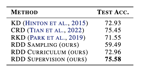
Figure 5: Final test accuracy(%) for resnet32x4→resnet8x4 on CIFAR-100.
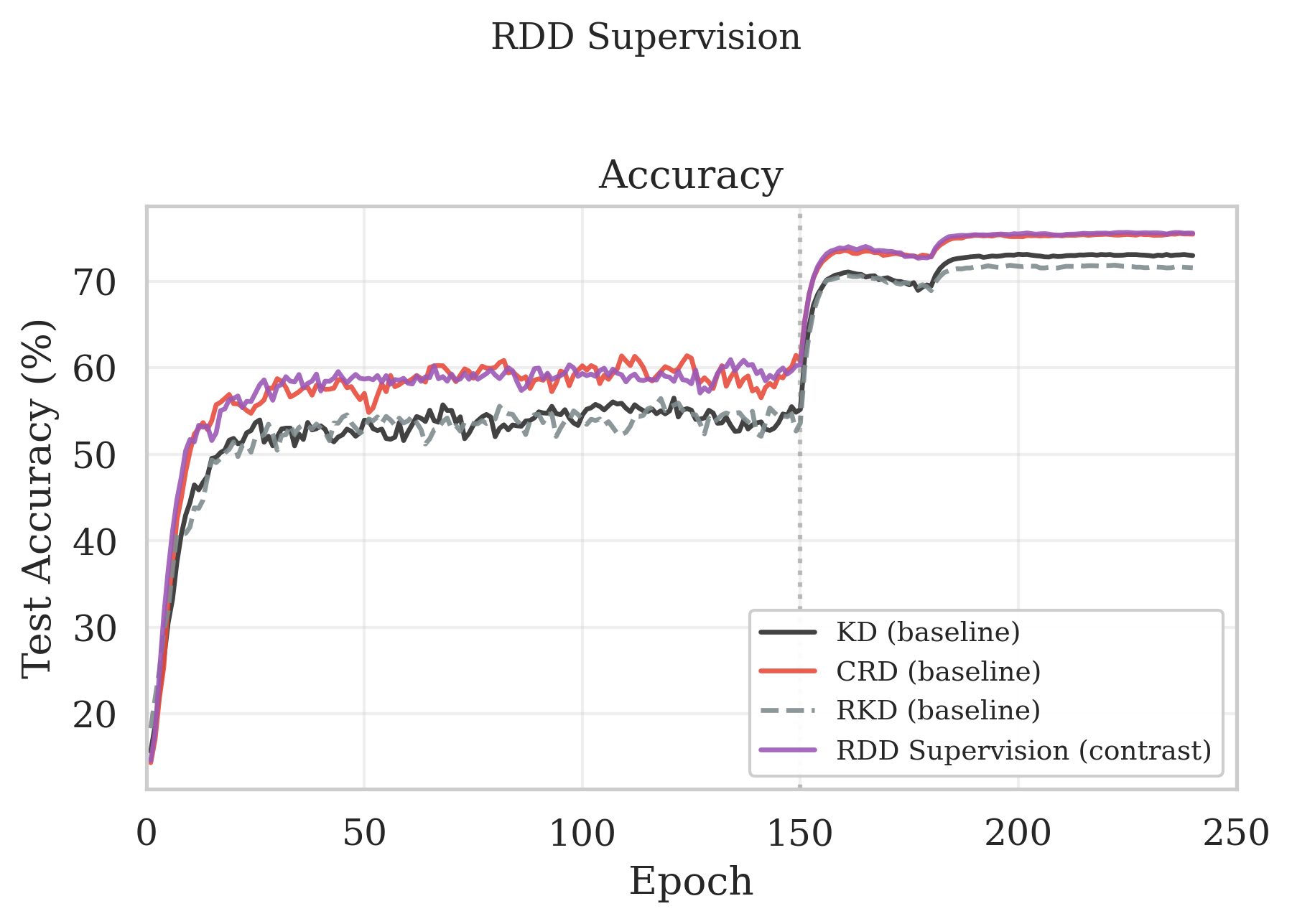
Figure 6: CIFAR-100 resnet32x4→resnet8x4 test accuracy. RDD supervision uses multi-negative contrastive distillation weighted by per-sample RDX affinity to emphasize teacher-student representational disagreement. Curves shown for KD, CRD, RKD, and RDD supervision.
#4. Discussion
- Weighting beats filtering, always: If you have a signal about sample difficulty, use it might want to bet on it to modulate your loss, rather than to exclude data.
- RDX staleness is a real problem. We refresh the affinity matrices every R epochs, but the student's representation evolves between refreshes. In early training when the student is changing fast, the affinities go stale quickly. We suspect an adaptive refresh schedule, triggered by shifts in the confusion distribution rather than a fixed clock, would help. We didn't solve this.
- The margin over CRD is narrow but consistent. 75.58% vs 75.45% is not a huge gap. What gives us confidence is that the gap appears specifically in the late-training region where targeted weighting should matter, and it reproduced across 5 runs. Whether this holds for cross-architecture transfers or at ImageNet scale remains open.
- The negative result is the most informative result. The 59.49% sampling collapse taught us more about distillation dynamics than the 75.58% supervision success. If your method can't survive data restriction, it's telling you something fundamental about the role of diversity in representation learning.
#5. Acknowledgments
I want to thank Abdulkarim Mugisha for working with me on this project. I would also like to Prof. Pietro Perona, for his guidance on experiments and paper writing, and Neehar Kondapaneni for his guidance and mentorship.#6. References
- [1]Hinton, G., Vinyals, O., and Dean, J. Distilling the knowledge in a neural network, 2015. URL https://arxiv.org/abs/1503.02531.
- [2]Park, W., Kim, D., Lu, Y., and Cho, M. Relational knowledge distillation, 2019. URL https://arxiv.org/abs/1904.05068.
- [3]Tian, Y., Krishnan, D., and Isola, P. Contrastive representation distillation, 2022. URL https://arxiv.org/abs/1910.10699.
- [4]Giakoumoglou, N. and Stathaki, T. Relational representation distillation, 2025. URL https://arxiv.org/abs/2407.12073.
- [5]Kondapaneni, N., Aodha, O. M., and Perona, P. Repre- sentational difference explanations, 2025. URL https://arxiv.org/abs/2505.23917.
- [6]Mindermann, S., et al. Prioritized Training on Points that are Learnable, Worth Learning, and Not Yet Learnt, ICML 2022.
- [7]Bengio, Y., Louradour, J., Collobert, R., and Weston, J. Curriculum learning. In Proceedings of the 26th International Conference on Machine Learning (ICML 2009), pp. 41–48, 2009.